Measurement FAQs

Irradiance is the measurement of radiant flux per unit area hitting or passing through a surface. An absolute irradiance measurement results in a spectrum that is accurate in both shape and magnitude. The y-axis scale becomes scaled in power or flux units like μW/nm or μW/cm²/nm, making it easy to calculate other power or energy values.

Measurements in absolute irradiance mode require a calibration using a source with known power output. A spectrum is measured with the sampling optic (fiber tip, CC-3 cosine corrector, etc.) connected to the calibration light source, and is then compared to the known output power of the calibration light source. Remember to always use the light source calibration file specific to the sampling optic being used, and calibrate just prior to measurement if possible.

The calibration process generates a file with energy response data for each pixel in the CCD, given in μJ/count. Factoring in the surface area of the sampling optic and the integration time allows irradiance measurements in μW/cm² to be reported (power=energy/time). Calibration is only possible if the absolute power output of the calibration light source is known, so if the light source calibration data is not given in the units μW/cm²/nm, it may not be a light source capable of calibrating for absolute irradiance measurements.

Calculating absolute irradiance takes into account the collection area of the sampling optic, and is corrected using the calibration data for each pixel, C_P.

I_P = (S_P - D_P) * C_P / (T * A * dL_P)

 where

C_p = Calibration file, in μJ/count (specific to the sampling optic)

S _p = Sample spectrum, in counts

D _p = Dark spectrum, in counts

T = Integration time, in seconds

A = Collection area, in cm² (A=1 for an integrating sphere)

dL_P = Wavelength spread (how many nanometers each pixel represents)

Q: How is CIELAB color space computed?

A: Typically, CIELAB is computed with some reference illuminant -- e.g., A, D65, or D75. These illuminants are normalized to a value of 100 at 560 nm. When doing a relative color measurement, the result is usually referenced to these illuminants:

Reflective/transmissive. The reflection or transmission spectrum (0-100% at each wavelength) is multiplied by this illuminant before the individual color values (X, Y, Z) are computed. Thus, the resulting X, Y, and Z values (which are the starting point for other color spaces such as CIELAB) are all relative to this normalized reference illuminant. That is, at no point can the reflection spectrum exceed the intensity (which shows up as the L* value in CIELAB) of the reference illuminant. The XYZ->CIELAB conversion (taken from CIE 15.2 1986, “Colorimetry”) bounds L* to the range of 0-100 as follows:

Given Y as the raw color measurement for the y-bar stimulus, and Yn as the corresponding raw color measurement for the reference illuminant, for large values of (Y/Yn), L* is computed as (116 * (Y/Yn)^0.33) – 16. The maximum reflectivity is assumed to be 100%, meaning that Y = Yn for all wavelengths. In this case, the formula for L* evaluates to (116 * (1)^0.33) – 16 = 100.

For small values of Y/Yn, the formula for L* changes to L* = 903.3 * (Y/Yn). If 0% reflection is the minimum, the smallest possible L* value is 903.3 * (0) = 0.

Emissive (relative irradiance). When we do color measurements from relative irradiance, the relative irradiance spectrum is also normalized (typically 100 at the peak wavelength for the ideal blackbody that is being referenced). When this spectrum is compared against a theoretical illuminant (e.g., D75) for the color measurement calculation, as described above for reflection, the magnitudes of the two spectra are comparable because both have been normalized to 100 at some wavelength. The calculations for L* are the same, but instead of multiplying a reflection spectrum against a reference illuminant to get the emissive spectrum, the relative irradiance spectrum is used directly. This keeps L* in approximately the same range of 0-100, though it could go slightly higher than 100 in some cases (i.e., if the sample was brighter than the reference at the wavelengths that contribute to the Y value).

That is, for reflection, transmission, and relative irradiance, it can be expected that the Y values will be approximately in the range 0-100, which translates to an L* value in that same range when computing CIELAB.

Absolute irradiance, however, is completely different.

In absolute irradiance, the spectrum is not normalized. That’s kind of the point — in the modes described above, the spectrum is always relative to something: a reference illuminant, a lamp that is assumed to be a blackbody source and so on, and by being normalized they are bound to some convenient limit (like 100). Absolute irradiance is not normalized to anything: the magnitude is computed in absolute terms against standard physical constants. The spectrum that results from an absolute irradiance calculation describes the light source being measured, and the magnitude is bound only by the possible intensity of that light source and the limits of the instrument. If you were to accurately measure the surface of a supernova with absolute irradiance, the total power (the spectral magnitude) would literally be astronomical. There is no bound of 100 anywhere. In other words, “100 for the brightest white” is all relative unless you mean “the brightest white that is possible in the entire universe”.

The fundamental problem is that the L* value in CIELAB is not an appropriate measure of absolute brightness. It might be useful for a reflective, transmissive, or possibly even relative irradiance measure of brightness, since these are relative. For absolute brightness, there is a whole other set of photometry measurements, including lumens, lux, candela, and luminance. These have no upper bound and are expressed (as absolute irradiance is) in standard physical units.

The reason that L* is being computed as being quite small is because the total amount of power (uWatts/cm^2/nm) being measured from the user’s monitor is quite small. Monitors do not produce much photonic power, which is what absolute irradiance is measuring.

If you were to do a relative irradiance measurement instead, using a white area of the screen as the reference, you might find that their L* value is in better agreement with what you expect. This would be true only because you would be making a measurement relative to something else; in this case, “the brightest white” that the display can generate, which becomes the definition of L* = 100 for the duration of that measurement.

If you wanted to see whether the absolute irradiance calibration was credible, you could try to measure daylight and compare that to the average solar irradiance for their part of the world. The average “insolation” (solar irradiance) reaching the surface is about 250 W/m^2, but this varies with latitude, time of day, and season. You may be able to look at the integrated power being measured across the absolute irradiance spectrum and see how it compares (though some unit conversion may be required).

Any time that a comparison is done between computer color spaces (typically RGB) and colorimetry based on models of human perception (typically XYZ, which leads to things like CIELAB) there is significant risk of error. RGB is usually nicely bound to 0-255 for each of its values. Conversion matrices have been created (with implicit and usually unstated reference illuminants and observers) to try to map from computer color spaces to human-model color spaces. These conversions are imperfect, and there are many cases where converting from one color space to another this way results in invalid color values. For example, the human-model color spaces cover a much larger range of colors and intensities than RGB can represent. Any time that a computer tries to convert between its own RGB colors into a human-model color space (such as CIELAB), one must be suspicious of the result. For instance, the “Digital Color Meter” application provided with some desktop computers is not necessarily authoritative on color measurement. It might be okay for relative color measurements (if the reference and dark spectra are taken as the brightest and dimmest the monitor can render — note too that “black” on a monitor will often still allow some of the backlight through), but it is not meaningful to use it for, or in comparison to, an absolute measurement of intensity.

Q: How do I determine divergence in single lens systems?

A: The divergence (a) of a beam focused using a single lens is tan(a) = d/f where f is the focal length of the lens and d is the aperture or fiber diameter.

Q: In probe-based Raman setups, what is the focal spot at the sample site?

A: For our RIP-RPB general-purpose Raman probes with 105 µm excitation and 200 µm collection fibers, the theoretical spot size is 158 µm with a 7.5 mm focal length or working distance. The depth of field is approximately 2.2 mm.

With the optional 5 mm working distance for the RIP-RPS stainless steel probes, the theoretical spot size is 105 µm with an approximate depth of field of 1.0 mm. Note that the actual spot size is about 20% higher due to spherical aberration. Additionally, the spot size highly depends on the sample properties. A reflective sample will have a spot size like the theoretical prediction and a shorter depth of field, whereas a transparent sample will have a larger spot size and greater depth of field.

Q: When making irradiance measurements, which mode should I use when comparing two scans?

A: Relative mode. Measurements taken with a single spectrometer are accurate relative to one another, even if the spectral shape is uncorrected. That means you can take the ratio of one emissive measurement to another and get an accurate change in the percent signal as a function of wavelength.

Here’s a good rule of thumb: Relative irradiance mode is needed when comparing measurements taken by different spectrometers, when determining the spectral shape, or when looking for peak location and shifts. Absolute irradiance mode is needed to quantify the amount of light.

Q: How can I reduce noise in my spectra?

A: You have several options available to you to minimize or eliminate the noise in your spectra?

Thermoelectric cooling. If you have a spectrometer (such as the NIRQuest and QE Pro models) that utilizes a thermoelectric cooler (TEC), be sure that the TEC and fan are enabled and set to the recommended setpoint.

Unprocessed mode intensity. The best measurements are made when the unprocessed mode intensity in counts is between 80%-90% of the number of counts where the detector becomes saturated. Check the region in which you are seeing the noise to establish if the counts are between 80% and 90% of where the detector becomes saturated (we use 85% as the “recommended peak value”). If the counts are much lower than this, please increase the integration time to get the signal close to or within this level. Please note that increasing the integration time increases the number of counts through the entire spectrum and, depending on the grating in your spectrometer and the light being measured, there may be some region that becomes saturated when the integration time is increased. Any pixels that are saturated will not yield good data. The data is scaled so that a spectrometer’s detector becomes saturated at 2 to the power of the number of bits of the A/D converter minus 1.

Scans to average. In OceanView, the “Scans to average” default is 1, which means that the spectrometer does 1 scan and that is your acquisition. The more scans to average you use, the greater the signal to noise ratio. Please note that your total acquisition time will be the number of scans to average multiplied by the integration time.

Boxcar averaging. Boxcar width is horizontal averaging, or averaging across the pixel array. This can help make your readings more coherent without increasing total acquisition times as standard averaging does. The number displayed (n) represents the single-direction width of the averaging, where 2n+1 is the total number of pixels being averaged (n pixels on each side plus the center pixel). Increasing this setting will reduce peak heights and is not recommended for Raman or LIBS type of measurements with strong, discrete peaks. However, for broad absorbance or fluorescence responses this can be highly useful with settings between 1 and 10; even a change from 0 to 1 will notably improve standard deviation at any given wavelength.

Integration time. As you increase integration time, the percentage of noise in the signal will increase. We define the maximum integration time of our spectrometers as that integration time where the noise comprises 50% of the total signal. Where feasible, use a larger diameter fiber to be able to use a shorter integration time.

Q: How do I calculate PAR (Photosynthetically Active Radiation)?

A: The amount of energy per photon at a given wavelength is computed as:

E = hc/L

Where:

    E is the total energy measured in Joules

    h is the Planck constant (6.626E-34 J*s)

    c is the speed of light (299792458 m/s)

    L is the wavelength of the photon measured in meters

Given that absolute irradiance is in units of uWatts/cm^2/nm, the conversion is as follows.

1. Multiply by collection area (cm^2): [µWatts/cm^2/nm] * cm^2 = µWatts/nm
2. Multiply by integration time (in seconds): [µWatts/nm] * s = µJ/nm
3. Divide by E (as computed above for this wavelength): [µJ/nm] / E = (photons * 10^6)/nm
4. Divide by Avogadro’s constant(A = 6.022 * 10^23): [(photons * 10^6)/nm] / A = µmol photons/nm
5. Integrate from 400-700 nm = µmol photons
6. Divide by collection area in m^2 = µmol photons / m^2
7. Divide by int. time in seconds = µmol photons / m^2 / seconds

Q: What is the best sampling device for my Raman measurements?

A: Raman spectroscopy can be performed on samples ranging from liquids and gels to powders, capsules, and large objects. A fiber optic probe assembly is the sampling optic most often used in a modular Raman spectroscopy system. It consists of a fiber bundle to route excitation light from the laser to the sample and collect Raman scattered light. Light at the laser wavelength (Rayleigh scattering) is rejected on the path to the spectrometer using a dichroic filter to avoid saturating the detector.

We offer a range of fiber optic probes for Raman spectroscopy with 532, 638, 785 and 1064 nm excitation. The RIP-series probes include models for laboratory, industrial and environmental applications with SMA 905 or FC connectors. The process probes are rated for use at up to 200 °C and 1500 psi, while the immersion probes go up to 500 °C and 3000 psi. Options include stainless steel and Hastelloy C housings and sapphire windows.

These probes mate well with the RM-LQ-SHS and OOA-RAMAN-SH sample holders, which are compatible with a variety of cuvette sizes and vials. RM-LQ-SHS has a magnetic cover, making it easy to load and unload samples, block ambient light, and improve the accuracy of Raman measurements. OOA-RAMAN-SH has a positioning screw that allows the user to adjust the distance between the probe and the sample simply and accurately to optimize the Raman signal while blocking ambient light with a cap. The OOA-HOLDER-RFA has many of the same features, but is designed as a multipurpose sampling fixture for Raman, fluorescence, absorbance and reflection measurements, with accessories for each technique. In addition, the RM-SERS-SHS holder is ideal for surface enhanced Raman spectroscopy (SERS) substrates that comprise nanoparticle chemistries on slides. This holder accommodates standard glass SERS slides and connects to a Raman probe. The RM-SERS-SHS provides accurate positioning for the Raman measurement, avoids the influence of ambient light, and improves the accuracy of the Raman measurement.

Q: How do I take the best reference and dark background spectrum for an absorbance measurement?

A: To take the best reference measurement, first allow the light source to come to thermal equilibrium (this can take up to 30 minutes in some cases). 

Ensure that all surfaces of the cuvette are clean and clear of fingerprints, dust, and dirt. Fill the cuvette with the exact solvent or buffer solution to be used for the sample, and check for bubbles. It is especially important to check for bubbles if using a transmission dip probe or flow cell, as they are prone to this source of error, particularly at the shorter path lengths.

Optimize integration time so that maximum signal is at ~80% of full scale and use the highest number of averages tolerable. Keep boxcar width to approximately the same value as the pixel resolution of the spectrometer, otherwise it can affect the spectral resolution.

Once the reference has been acquired, go into transmission mode and take a look at the resulting spectrum. If a good quality reference spectrum has been stored, the transmission of the reference solution should be at 100%, with some noise around this value. Wavelength regions with more noise indicate the wavelengths at which accuracy will be the least for the sample measurement (typically the shortest and longest wavelengths).

When taking a dark measurement, it is best to block the light at the light source if possible. Turning the light source off and then on again will throw the light source out of thermal equilibrium and require a new reference measurement. Alternatively, many cuvette holders have a filter slot where the light can be blocked. Just be sure to use a piece of metal or another object that is guaranteed to be 100% opaque. Paper, even cardboard, can be deceptively transmitting, and it only takes a very low level of light to affect a measurement.

A relative irradiance measurement corrects the shape of a measured spectrum without defining the scale. It simply scales it from 0 to 1. Calibration is performed by sampling a blackbody light source of known color temperature. The software then uses the color temperature to calculate the theoretical spectral shape of the source and apply a wavelength-by-wavelength correction to the full spectrum.

Calculating relative irradiance looks a lot like a transmission calculation, with the addition of the blackbody reference shape, B(λ).

where:

B(λ) = Theoretical shape of reference (blackbody equation)

S(λ) = Sample spectrum, in counts

D(λ) = Dark spectrum, in counts

R(λ) = Reference light source spectrum, in counts

Q: What is the order of operations for spectral calculations in Ocean Insight software?

A: Please follow these simple steps for spectral calculations:

1. Set Integration Time.
2. Average multiple scans (averaging will lower the overall noise for the subsequent steps).
3. Subtract Dark(bias). Dark subtraction is important for linearity and stray light correction. Make them as close to a zero baseline as is practicable.
   1. Enable Electrical Dark Correction (if available)
   3.2. Take a Dark and a Scope minus Dark
4. Correct for detector non-linearity.
5. Correct for stray light(optional).
6. Apply Boxcar Smoothing.
7. Take a new Dark subtraction
8. Start making measurements.
   
   

Note: If you change the Integration Time, Averaging or Boxcar Smoothing, you must take a new Dark (Bias) subtraction. This is done while the Linearity Correction is enabled.

Q: What is the relationship between spectrometer slit size and optical resolution?

A: Optical resolution of a monochromatic source -- measured as Full Width Half Maximum (FWHM) -- depends on the groove density (mm^-1) of the grating and the diameter of the entrance optics (optical fiber or slit). In configuring your spectrometer, consider two important trade-offs:

• Resolution increases with an increase in the groove density of the grating, but at the expense of spectral range and signal strength; and
• Resolution increases as the slit width or fiber diameter decreases, but at the expense of signal strength.

The slit is the small opening that allows light to enter the spectrometer. The slit width is inversely related to the optical resolution of the spectrometer such that smaller slit widths will produce greater resolution. A smaller slit, however, allows less light into the spectrometer. For most Ocean Insight spectrometers, the slit height is 1000 μm and only the width varies (from 5 μm up to 200 μm). For spectrometers with no slit, the diameter of the optical fiber limits the amount of light entering the system and performs the function of the slit.

Download Quick Start Guide - Changing the Slit

Q: How do I determine the spot size of my sampling setup?

A: Let’s use the drawing below to demonstrate how to get to your answer. In this example, the distance (“X” on the drawing) is 3 inches.

First, we calculate the half angle (12.7°) of the fiber, which is based on its numerical aperture and index of refraction in air. The NA of our optical fibers and probes is 0.22 +/- 0.02 and yields an acceptable angle of 25.4° in air.

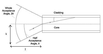
Considerations:

Numerical Aperture formula

                        Na =  Л Sin(θ)
                        θ = Sin^-1 (Na/ Л)
                        θ = Sin^-1 (0.22/ 1.00033) = 12.7°

Given that …

Numerical Aperture = 0.22
Л (Index of refraction in air) = 1.00033

X (Distance) = 3 inches
h (Height, or the distance from the tip of the fiber or probe to the sample surface) =?

θ (Half Acceptance Angle) =?

Since …
                        Sin(θ) = (h/X)
                        h = X Sin(θ)

And …

                        Spot Size = 2h

Then…
                        Spot Size = 2(X Sin(θ))

                                      = 2(3 Sin (12.7°))
                        Spot Size = 1.32”