Setting up your irradiance calibrated spectrometer to measure lamp output power

IMPORTANT: PLEASE REFRESH YOUR BROWSER IF YOU DO NOT SEE ANY IMAGES/SCREENSHOTS ON THE PAGE.

1. Save to your computer the calibration file that came with your calibrated spectrometer.

2. Connect your spectrometer to your computer.

3. Launch OceanView software and select the Spectroscopy Application Wizard option from the Welcome Screen or open the Spectroscopy Application Wizard by clicking on the OceanView icon in the upper left corner of the software window.

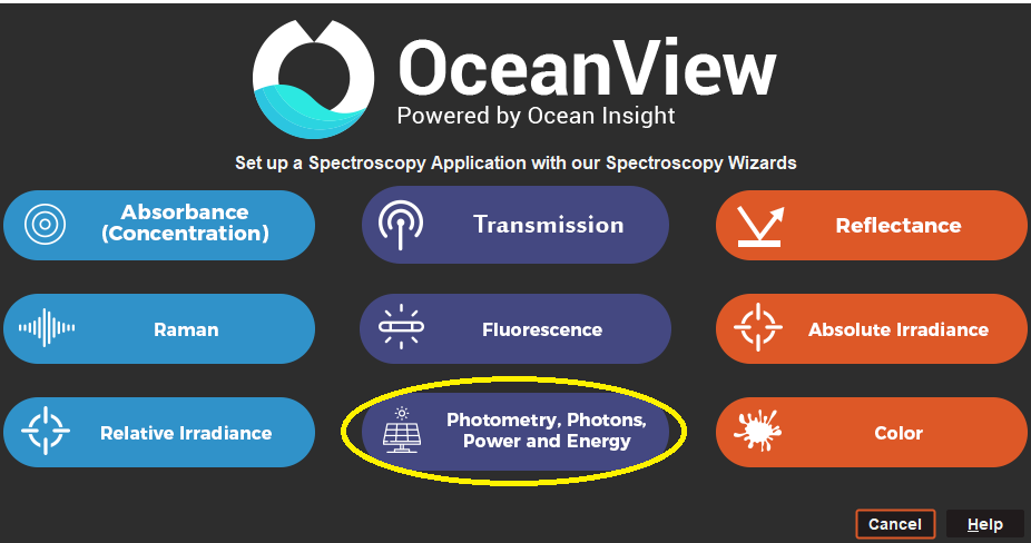
4. Select the Photometry, Photons, Power and Energy Spectroscopy Wizard.

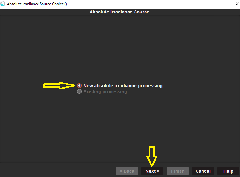
5. Select | New absolute irradiance processing | and click Next.

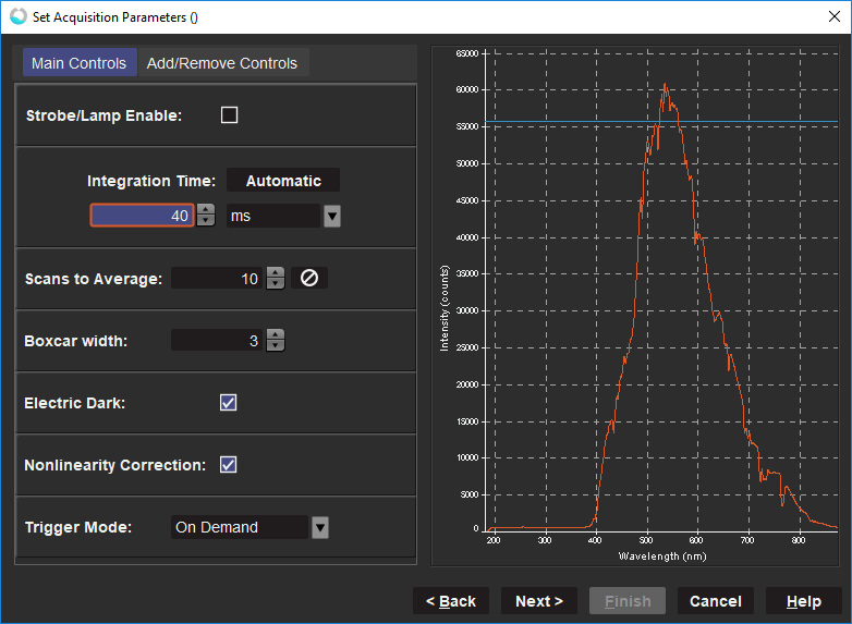
6. With your light source on and illuminating your spectrometer collection optics, set up your acquisition parameters:

a. Integration time: Integration time is the period of time over which the spectrometer collects photons. We find that the best measurements are made when the signal intensity is between 80% and 90% of its full intensity range (which is indicated by the horizontal line in the graph on your Set Acquisition Parameters Wizard step). Be careful not to allow any pixels to become saturated, as saturated pixels will not provide useful data. Increase your integration time to increase your signal and decrease integration time if you are saturating the spectrometer, as seen by a spectrum with a flat top at the maximum intensity for your spectrometer.

b. Scans to Average: This feature specifies the number of discrete spectral acquisitions that the device driver accumulates before OceanView displays a spectrum. The higher the value, the better the signal-to-noise ratio (S:N). The S:N will improve by the square root of the number of scans averaged. Note that the total measurement time is the integration time multiplied by the number of averages. For example, using a 100 msec integration time with 10 averages would give a 1000 msec total measurement time until your spectrum is displayed in the software.

c. Boxcar Width: Use this to set the boxcar smoothing width, which is a technique that averages across spectral data. This technique averages a group of adjacent detector elements. A value of 5, for example, averages each data point with 5 points to its left and 5 points to its right. The S:N will improve by the square root of the boxcar width value. The higher the value, the better the signal-to-noise ratio (S:N). Note that if this value is set too high you may smooth important spectral features, so choose your value carefully.

d. Electric Dark: This feature should be enabled by default if available for your spectrometer.

e. Nonlinearity Correction: Enable if available for your spectrometer.

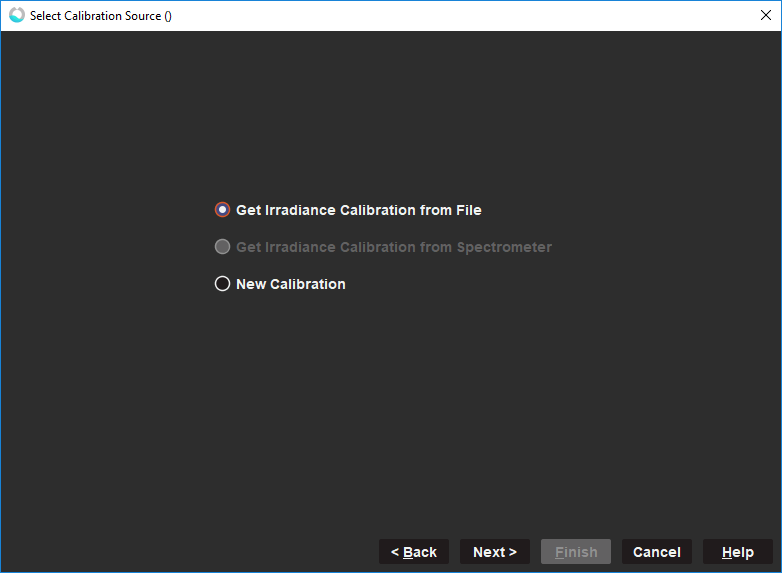
7. Click on Next to go to the next step in the Wizard. Select | Get Irradiance Calibration from File | and click on Next. 

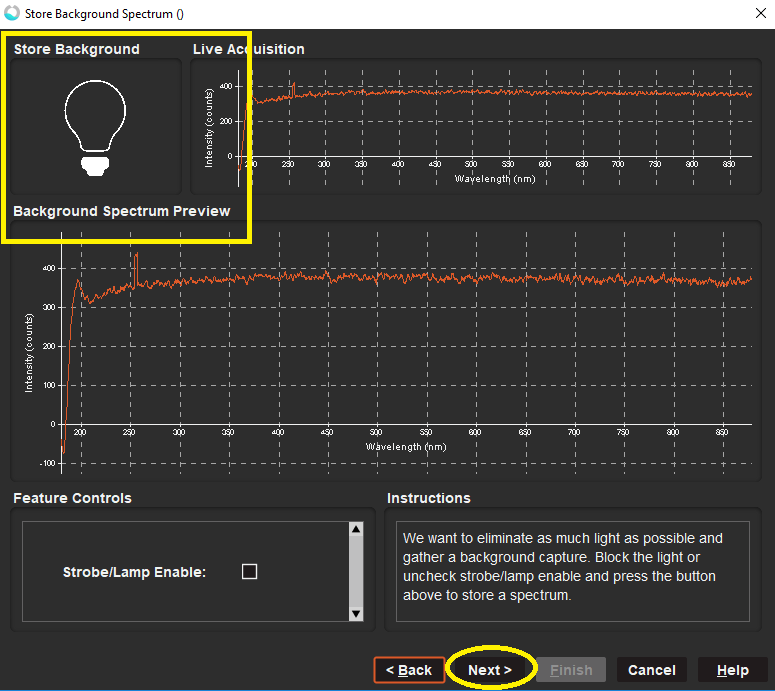
8. Store Background spectrum by blocking the light entering your collection optics and clicking on the light bulb, then select Next. It's important not to turn off your properly warmed up light source for this step, as doing so can affect lamp stability.

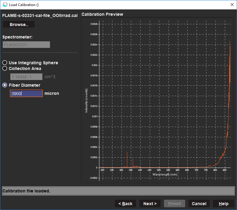
9. Browse to the *OOIIrrad.cal calibration file that came with your radiometrically calibrated spectrometer and load it, then click Next.

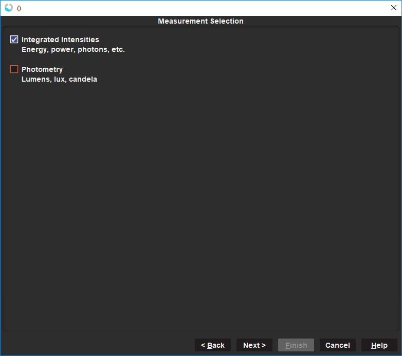
10. For this example, we’ll select the power option – Integrated Intensities.

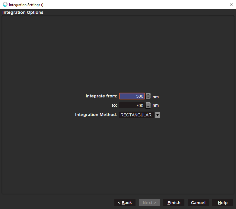
11. Select your wavelength range and integration method, then click on Finish. The wavelength range set in this step will determine the wavelength range over which your output power is calculated. For example, to calculate the power output in the UVC range only, you would integrate from 200-280 nm (depending on how you define the UVC wavelength range).

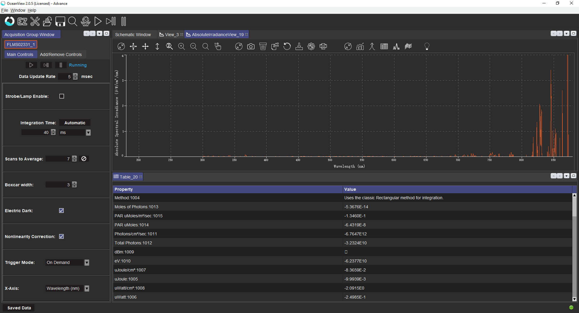
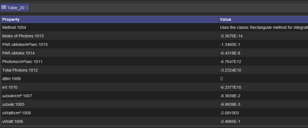
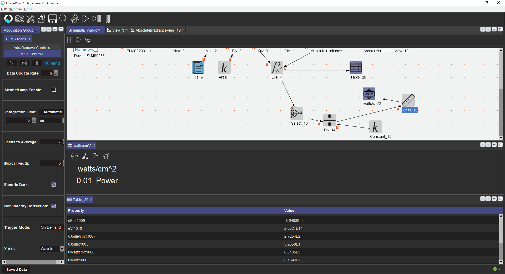
12. After you complete the Wizard, an Absolute Irradiance graph will open along with a table showing all the different Photometry values output by OceanView for the wavelength range specified in the Integration Options step of the Wizard.

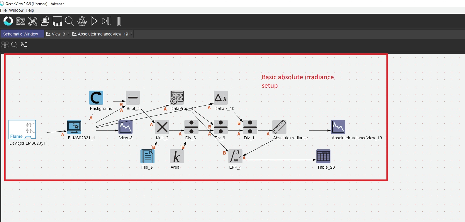
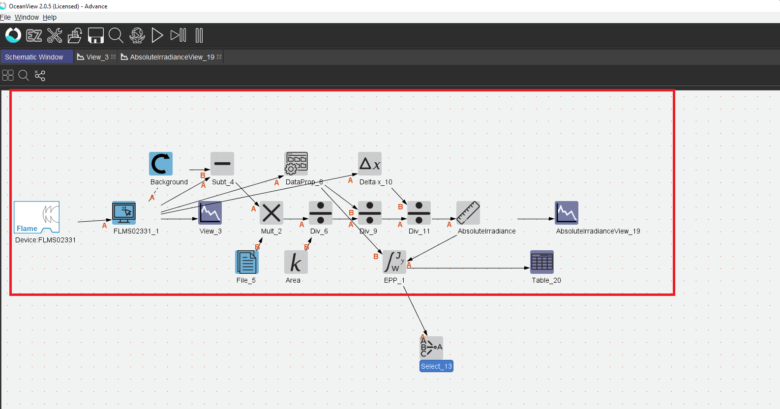
13. If the power value of interest is not included in the table or if you’d like to see one of these power values displayed by itself in a separate window, you will need to customize the Absolute Irradiance Schematic. When you open the Schematic, you will see the nodes for the basic Absolute Irradiance processing created by the Wizard.

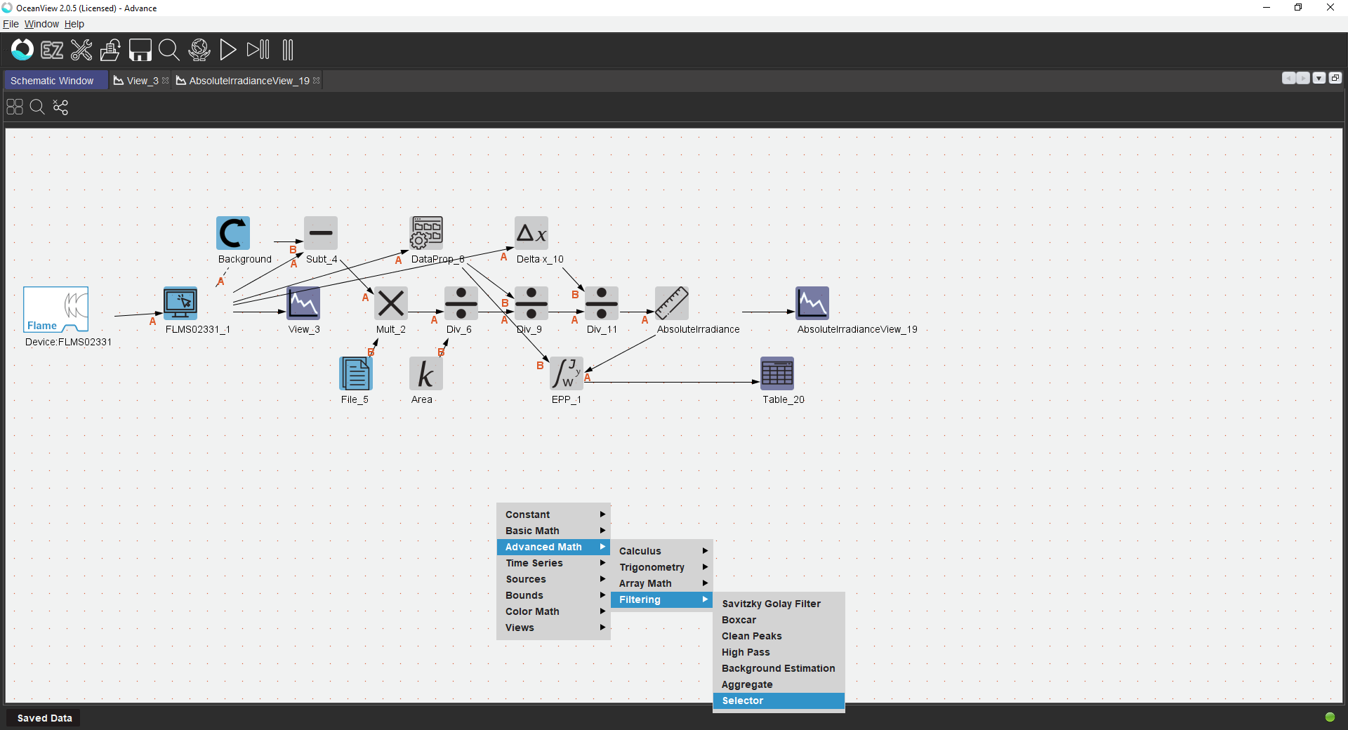
14. To select just one value from the table of power values to display in a separate window, right-click on an empty space on the Schematic to bring up the menu of available nodes.

Go to Advance Math -> Filtering -> Selector

15. CTRL+CLICK and drag an arrow from the Photometry node to the Selector node

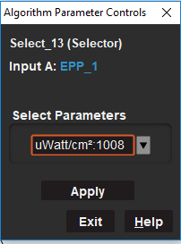
16. Double-click on the Selector node and select the value you wish to display or alter to calculate a different power unit. In this example, the uWatt/cm² value is selected. To display this value in a separate window, skip to step 21. To convert the power value to some other unit (W/cm² in the example below), continue with step 17.

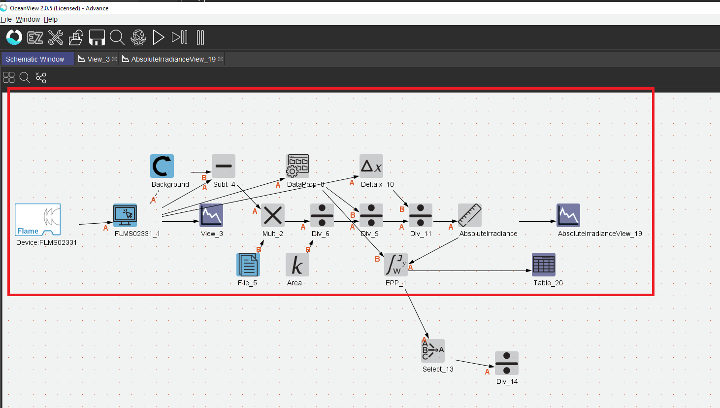
17. You have several options available to convert the selected power unit to a different unit (for example, change from uWatt/cm² to Watt/cm²). To add the calculations needed for unit conversion to the Schematic, right-click on an empty space on the Schematic and go to: 

Basic math -> Divide

18. In this example, we are using a Divide node to convert the power units from uWatt/cm² to Watt/cm². Note that many other nodes are available in the Basic Math menu (accessed by right-clicking an empty spot on the Schematic) to enable you to convert the standard units output by OceanView to the power units of interest. Connect the Divide node to the Selector node by CTRL+CLICK and dragging an arrow from the Selector node to the Divide node.

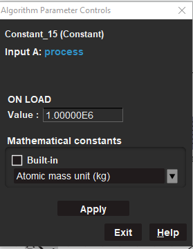
19. A Constant node is used to convert the power value by whatever factor is required. Right-click on an empty space on the schematic and add a Constant node.

Constant -> Select Constant

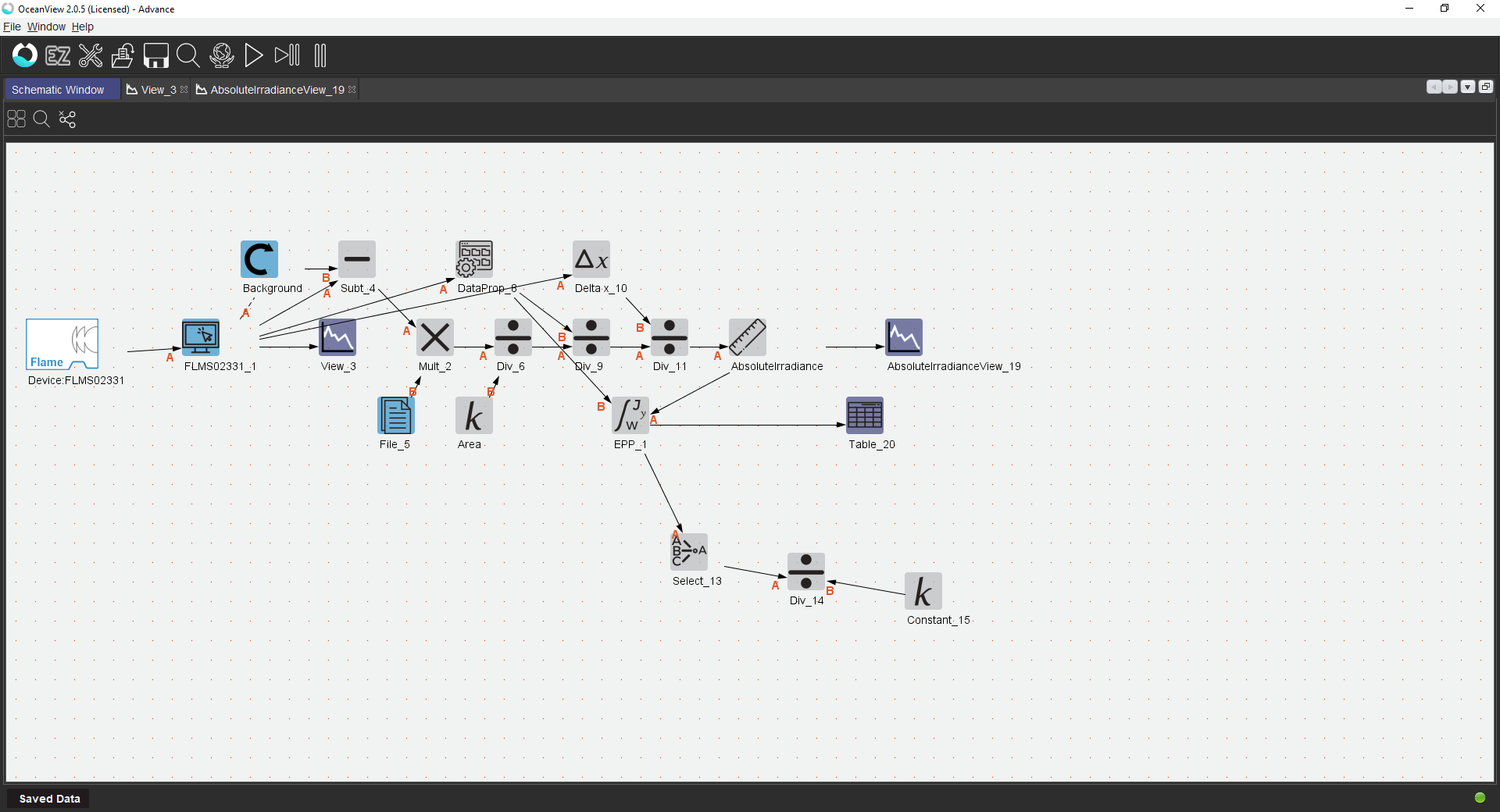
20. Double-click on the Constant node and enter the value needed to convert your power unit, then click Apply. For this example, converting from uWatt/cm² to Watt/cm², we used a value of 1,000,000 for the conversion. Connect the Constant node to the Divide node by CTRL+CLICK and dragging an arrow from the Constant node to the Divide node.

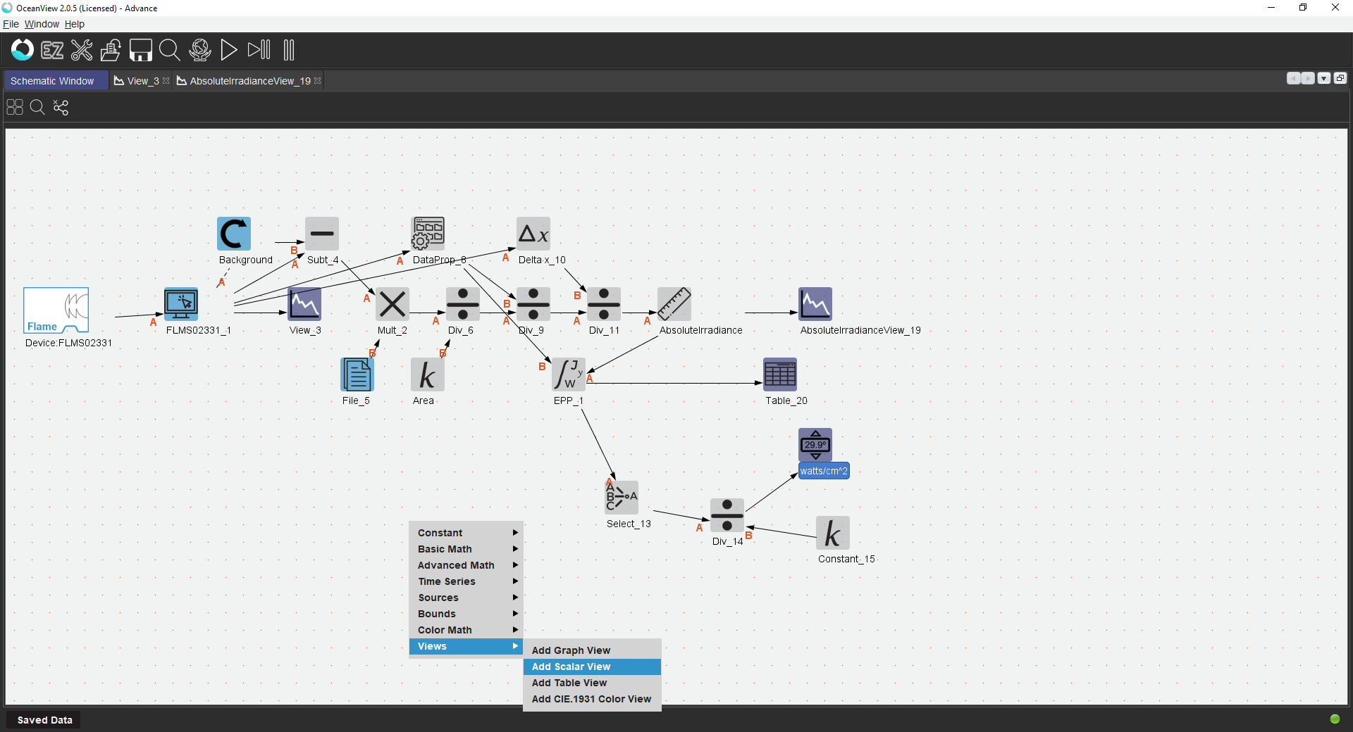
21. To display your desired power unit in a separate window, add a Scalar view node to the Divide node by right-clicking on empty area in the Schematic and going to: 

Views -> Add Scalar View

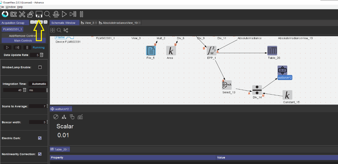
22. You can rename your Scalar view node by right-clicking on the Scalar view node.

23. You can also add a Unit Label node to the Divide node to label the data in the Scalar View window. Right- click on an empty area in the Schematic and go to: 

Constant -> Unit labels -> Connect the Unit Label node to the Divide node -> Double-click on the Unit label node and provide a label for the data displayed in your Scalar View.

24. Be sure to save this Schematic as a project, so you can quickly reload it the next time you open OceanView. To save this Schematic, click on the diskette icon and save the project to your computer.

For more on OceanView startup wizards and schematics, we recommend Part 2 of our Best Practices for Using OceanView webinar series.